Improved hall effect encoder performance

moteus first added support for hall effect encoders way back in 2022, when many new encoder types were added. At that time, hall effect sensors were treated basically like any other encoder. However, because of their inherent low resolution, this resulted in them performing much worse than other encoder options, especially at low speed. In practice, very careful tuning of the encoder low pass filter was required to achieve useful performance and that performance would often only be valid in a narrow range of speeds.

Now, as of release 2025-07-21, moteus has a suite of new heuristics which drastically improve the performance of hall effect encoders at all speeds, and make them relatively insensitive to filter bandwidth selection. If you don’t care about the details, just upgrade your firmware following the instructions in the reference manual and be on your way! If you do care about the details, read on for more.

Why hall effect sensors are different

Most encoders used for positioning of motors, like the onboard on-axis magnetic encoder included with all moteus controllers, have a relatively high resolution compared to the range of motion. For instance, the AS5047P used on moteus-c1, has 16384 possible reported counts for a single revolution (although practical accuracy is less than this). Capacitive, off axis magnetic, or inductive encoders similarly typically produce thousands to millions of counts for a single revolution of a shaft.

As described here, moteus has to use encoders for two purposes. For usage with the ouput position control loop, both position and velocity are needed, and the accuracy of the position and velocity directly corresponds to the overall control performance that can be achieved. In contrast, when using an encoder for commutation only position is needed, and the accuracy only has to be just enough to identify where in the electrical phase the motor is. For low pole count motors, that can be very coarse.

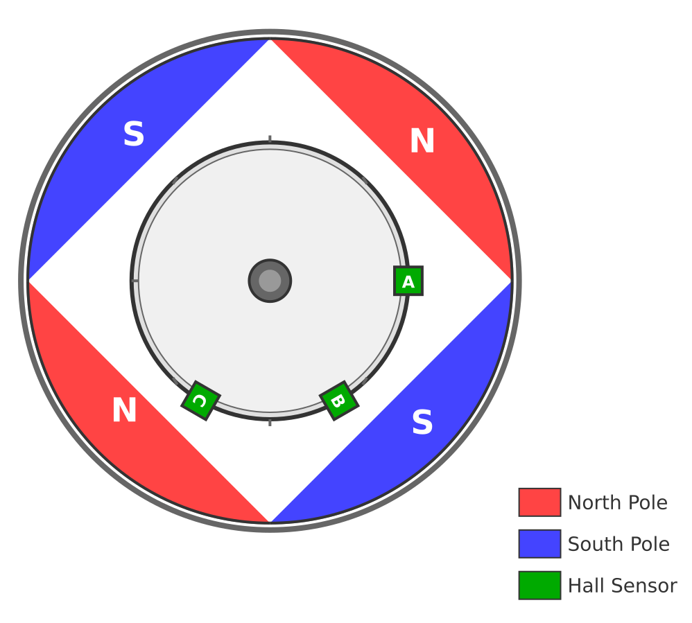
Hall effect encoders often integrated into brushless motors are designed primarly to achieve this latter commutation function, and thus count exactly 6 times for each electrical revolution of the motor. They accomplish this by positioning 3 “hall effect” magnetic field sensors such that they either detect the actual rotor magnets, or an auxiliary multi-pole magnet ring affixed to the rotor.

For, say a 8 pole (4 pole pair) brushless motor, this results in an encoder waveform that increases through 24 counts for a single revolution of the rotor. Here is a plot comparing that resolution with an encoder that shows the rough effective resolution of an AS5047P encoder. The steps in the AS5047P are there, but are so small that you cannot really distinguish them.

Thus you can see that the effective resolution available from hall effect sensors is much lower. It is not always as extreme as the plot above, as some hoverboard motors have 15 pole pairs, or 90 measurable encoder counts per revolution, but still, it is much worse.

How moteus used hall effect sensors previously

The initial implementation of hall effect sensors treated them exactly the same as all other sensors. At each control cycle, the current value of the encoder was used as the input to a digital PLL filter. Since the control loop runs at a default of 30kHz, that means with low resolution hall effect sensors, the same value is fed in over and over again until, eventually, a different value is repeatedly fed in.

This never gives “good” results, but depending upon the low pass filter bandwidth configured, it can give “less bad” results. Particularly, the reported velocity is very poor and “spiky”. This is because the filter calculates that the velocity is 0 with each update at the same position, and then calculates a very large velocity at the moment of transition, which then ramps back down to 0 rapidly as the position stops changing.

In this plot, the dashed lines are a “ground truth” estimate of the velocity and position whereas the solid red line is the PLL filter’s estimate of the velocity. When used as the input to the position PID controller, you can see how this velocity would be challenging to tune for stable control.

The “solution”

There have been many approaches to using low resolution encoders in control systems. If only very low speed operation is required, the velocity can just be estimated by measuring the time between changes in the encoder value. However, that gives poor results at higher speeds when there is insufficient resolution in the measurement of time - this is when the current PLL filter approach works well. The approach I used was to dynamically switch between the two modes depending upon the inter-sample timing. Further, the digital PLL formulation is tweaked to only update the velocity (but not position) when a new sample has arrived, which further decreases the velocity error. This was inspired by the PicoEncoder, although the actual implementation here differs in many ways since it still needs to work with encoders that have significant noise and also high resolution ones.

While the above principle seems straightforward, a fair number of heuristics were required to make it work in practice. Complications arose from the non-uniformity of angular spacing of the hall sensors, interactions from the outer control loops and just artifacts from the dynamics of operating at low speed or with large accelerations. Let me try to document some of them here.

Transition point: In order to switch to PLL based operation when the speed is high enough, some threshold must be used. The threshold chosen by moteus is set to be 1/4th of the 3dB cutoff time constant. So for a 100Hz cutoff, any intervals that are closer than 2.5ms will result in a switch into PLL based operation. If this is set too low, then slow mode will be engaged too long, resulting in large errors in velocity at high speed. If it is set too high, then the PLL filter will be engaged too long, resulting in pulses of velocity at low speed.

To help evaluate this, I created a tool which applies sine waves of varying frequencies, discretizes them as if they were hall sensors, then passes them through the encoder processing stack. It then measures and plots the observed gain at different frequencies and compares it with the ideal filter response from a pure PLL filter.

That shows that if the transition point is too large, in this plot anything at 0.5 or higher, then undesirable artifacts start appearing at low frequencies.

Problems with having a transition point too low can be seen in time domain plots and noise metric comparisons. In this plot with a 100Hz filter cutoff, the velocity is ramped from near 0 to a large negative value. With a transition point of 0.25, the PLL filter engages at around 400 counts per second, but with a transition point of 0.10, it must reach ~900 counts per second to engage.

Hysteresis: When switching from the PLL mode to the transition timed mode (“slow” mode), a hysteresis count is used to prevent temporary transitions into the slow mode. Currently, 3 samples greater than the transition threshold must be observed before switching. Realistic motors have non-uniform spacing between hall sensors, such that even at a constant speed the inter-sample timing can be above and below the transition threshold during one electrical revolution. Switching back and forth rapidly between the two modes does not yield good results, especially when operating at speeds very near the transition point. This plot shows a zoomed in version of the above time domain sequence, with orange showing the filtered value with hysteresis and blue showing without. In this case, the blue value intermittently uses the slow mode for longer.

Direction changes: When changing direction, it is common for any discrete encoder to have a short “blip” reading in the old direction before moving back. If time between transitions were used simply, that would result in reporting a very large velocity temporarily. Instead, in any instance where the direction changes, the velocity is forced to 0 until a second transition in the same direction is detected. The below plot shows the effect of this on a dataset where a motor was moved by hand very slowly such that it occasionally came to a near stop. In those cases, the position occasionally made one tick in the opposite direction. The dark blue velocity line shows the velocity without 0 being forced, while the thinner orange line shows the effect of forcing the velocity to 0 in such situations.

Slowing to a stop: Transition timing works well at slow speeds, but does have a problem with deceleration at low speed, particularly so if the deceleration is all the way to a stop. At that point, no further transitions will ever be observed. In a straightforward implementation, the estimated velocity will remain non-zero indefinitely. To address this, when the filter detects that the propagated position has advanced beyond certain thresholds, the estimate of speed is reduced exponentially. Beyond a first threshold the reduction is with a 120ms time constant, and beyond the second threshold the reduction is with a 20ms time constant. This ensures that the reported velocity reaches 0 relatively quickly after a stop actually occurs, and is a tradeoff between adding additional velocity noise in during periods of normal deceleration.

This plot shows how the thin blue velocity estimate decreases to 0 after the position input stops advancing. It first decreases at a slow rate, then increases at a faster rate as the position proceeds further.

Commutation: When the hall sensor is used for commutation, a number of additional heuristics are activated. When not used for commutation, it is acceptable for the estimated position to be off by more than 1 count, but when used for commutation, this is basically never the case. The most common reason for permitting the position to deviate by more than a single count when not used for commutation is when operating well beyond the low pass filter bandwidth, for which the reported position and velocity can deviate arbitrarily far from the sensed value.

Thus there are a few places where the position is forced to a new value or limited to ensure that it is never more than 1 count away from the current sensed value. Since this does neuter the low pass filter, a workaround is available if the filter is necessary for position control. Just configure the same hall effect on two different motor_position sources, one used for commutation and the other for output.

This plot shows the same source data processed two ways, with one output run configured as a commutation source and the other as output. For position, the thin red line is the commutation source and can be observed to track the source position within 1 value. However, because it is tracking faster than the filter bandwidth, the commutation velocity, shown as thin orange, tracks very poorly. The output configured run, with thick green position tracks poorly, whereas the velocity in thick blue tracks somewhat better. In general, you don’t want to be operating a system mechanically far beyond the configured filter bandwidth, so this is most academic.

Future work

Currently, all of these heuristics are only applied to hall sensors, and not to other potentially low resolution sources like a generic quadrature input. If someone finds a use case where that matters, then I will think about adding in a mechanism to either always enable these methods, or more likely, add a configurable knob to do so.

Usage

To take advantage of the better performance, all you have to do is have a new enough firmware. No additional configuration is necessary, it should just work.

It is the case that if moteus_tool detects a newer firmware, it will no longer artificially lower the encoder filter bandwidth for hall sensors, but if the hall effect is used for commutation (likely), then this doesn’t really matter anyways.

Good luck!