Moteus performance analysis tool - v2
Well, that didn’t take long! Only a short time ago I announced the first release of the moteus performance analysis tool. In that short time frame, I basically did a complete rewrite (more on that later on), that added a bunch of new capabilities. You can now create nearly any table comparison you can imagine, enter custom motor configurations and even produce 2D graphical plots showing supply power, temperature, or efficiency versus speed and torque. Check out the tool live here, and read on to learn more.
There are a whole lot of new features and capabilities here, let’s break them down one by one.
New user interface
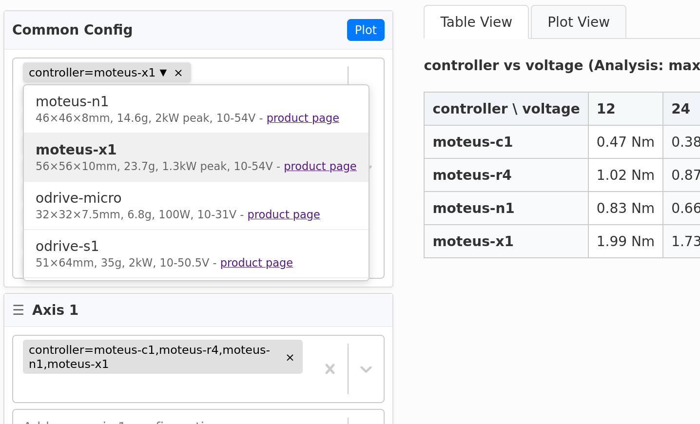
The first thing you’ll notice is the entirely new UI:
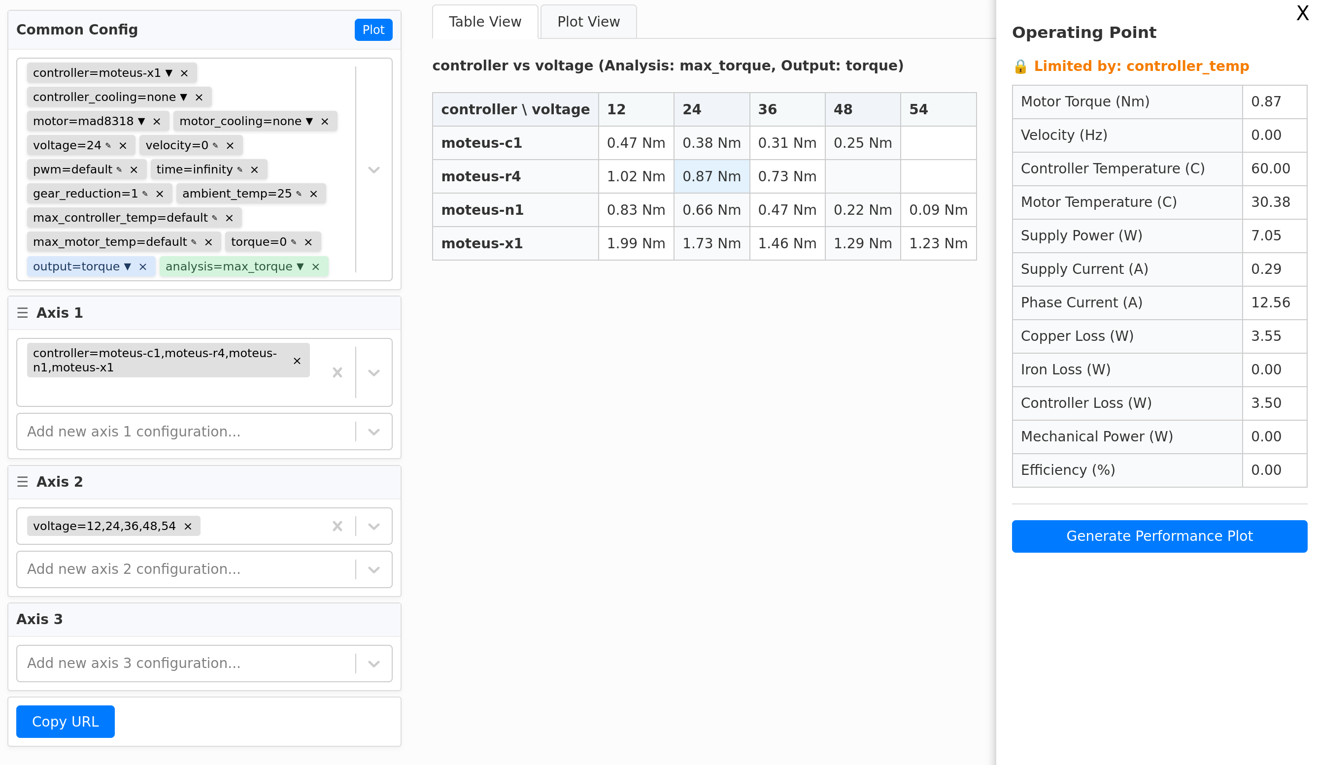
It has roughly the same structure as before, with left panels that allow configuring the analysis, a center area to display table results and a right side overlay for detailed information. However, the configuration area is significantly different. Instead of having one “panel” per possible configurable variable, now there are generic edit fields filled with “chips”, where each chip represents a single configurable value. That allows many more configurable variables to be shown in the same user interface space.
Chips are entered by typing, with auto-complete, into the edit field. After the equal sign, either a number, a constrained value, or for axis chips a comma separated list of those can be entered. Chips can be edited in place with a drop down for those with constrained values, or by clicking to create an inline edit field.
The pane configuration is the next big obvious change. Instead of automatically selecting which variables are rendered on which axes, you now can directly configure the variables to compare by placing chips in the axis panels. Each line in the axis panel will result in another row/column of a table. If commas are used between values, that is internally treated as if it were multiple lines. If multiple values have commas, then that axis gets the cartesian product of all things with commas.
This construction allows you a lot of flexibility. The default axis configuration shows a simple example, where one table axis has a variety of controllers and the other has a variety of voltages. The configured analysis is to find the maximum torque and the output variable is that torque. However, since all of those configurable things can be placed in axis edit fields, you could just as easily compare the maximum torque vs the maximum speed at a fixed torque vs the supply power when operated at a specific speed and torque.
Each of the axes can be dragged around to change their order, which lets you get exactly the comparisons you want shown. That’s especially helpful with more than 3 axes, as then multiple tables are generated.
Further, all of this configuration can still be distilled down into URL query parameters, so that the “Copy URL” button produces a URL that will replicate whatever analysis you have achieved.
Feasibility and constraint diagnostics
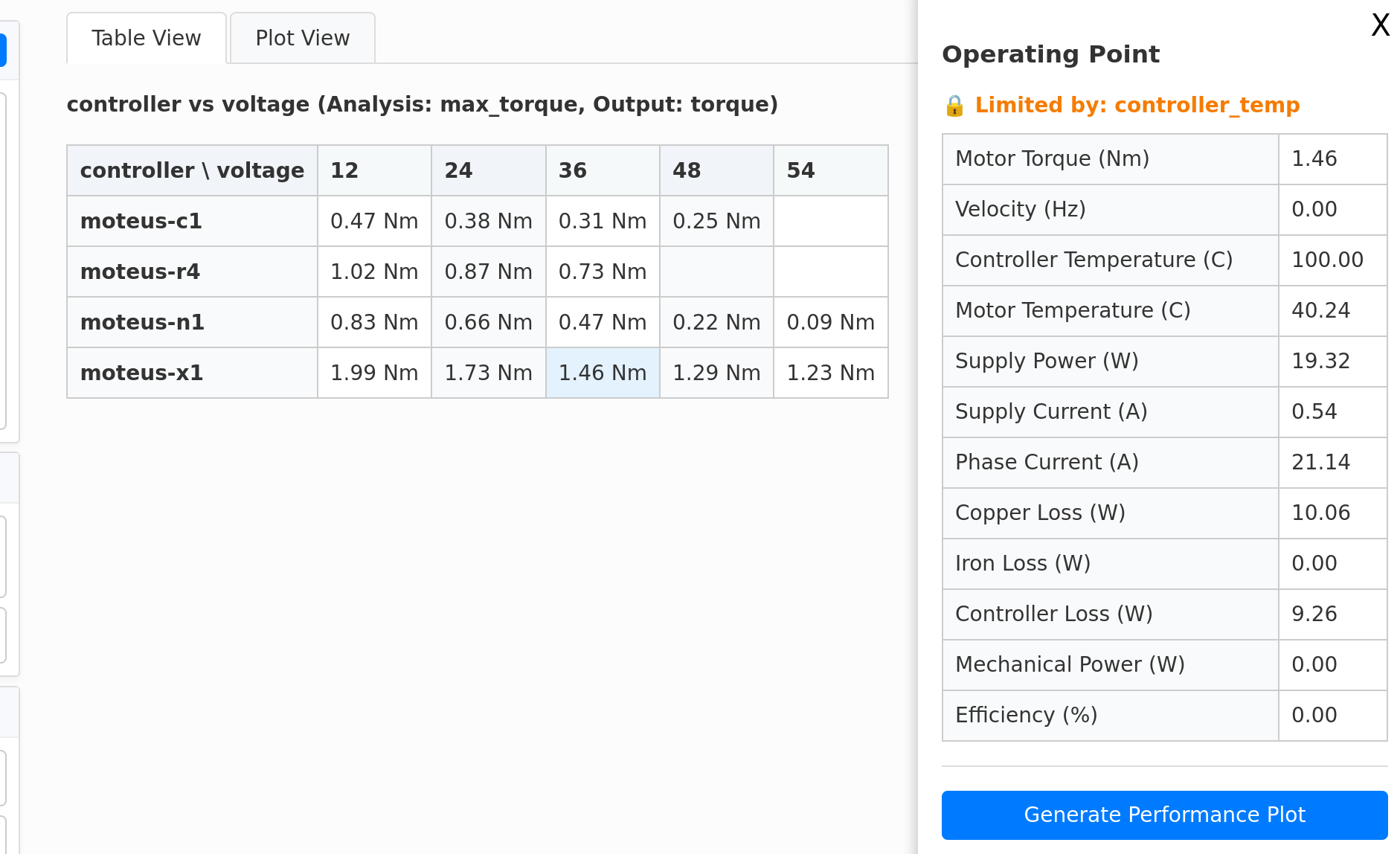
When an operating point analysis results in a violation of one of the system constraints, the table still shows the result, and the operating point overlay now displays a textual reason for the violation:
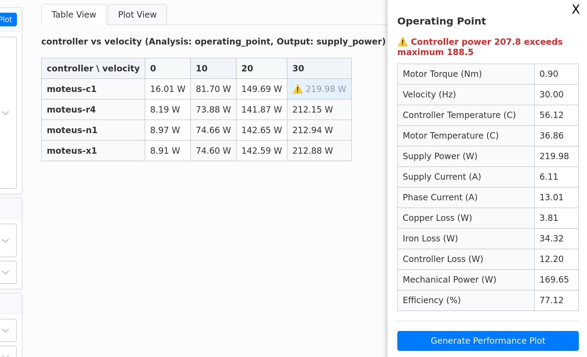
When constraint analysis are performed, the operating point window will tell you which parameter was the limiting factor for that particular constraint point. You could often figure this one out on your own by looking for which operating point value was saturated, but it is a lot easier to reason about if you don’t have to guess.
New configurable parameters
All of the configurable parameters available before are present, plus some new ones:
- gear_reduction: A gearbox can be configured. All velocities and torques are reported at the output of this reducer, so it can be used to estimate performance with actuators that have a reducer installed.
- max_controller_temp: When set to “default” this uses the factory set default maximum temperature for the current controller. However, you can raise or lower it to see the effect.
- max_motor_temp: Similar to
max_controller_tempthis lets you override the motor maximum temperature. Given that most motors don’t quote a maximum rated temperature, the one used in mpat is mostly a guess anyway, so this lets you decide for yourself. - analysis=max_velocity: This performs a constraint optimization to determine the maximum speed that can be achieved while satisfying all other configured parameters, including torque, thermal time duration, cooling, etc.
- analysis=operating_point: This just evaluates the system at the configured torque and velocity.
- output=(many): In the old version of mpat, the value that could be displayed in a table was relatively limited. If you performed a maximum phase current analysis, the output could be only phase current. If you performed a maximum torque analysis, the output could only be maximum torque. The same for the other analysis types. Now, the output can be any of the values available from the operating point analysis no matter what analysis type is used. That includes torque, velocity, controller temperature, motor temperature, supply power, supply current, phase current, copper loss in the motor, iron loss in the motor, mechanical power, or overall efficiency.
Parameterizable motor model
Maybe the biggest new configurable parameter is the motor=model option, which allows you to manually enter parameters for an arbitrary motor. It isn’t that great, as the parameters needed are rarely all available on datasheets, but it is at least a start. To use it, any field that has a motor=model configuration enables a number of additional configuration options:
- motor.kv: The normal Kv value, as read from datasheets
- motor.r: The phase to phase resistance in ohms
- motor.l: The phase to phase inductance in henries
- motor.thermal_r: The R term for a lumped single-joint thermal model between the motor and ambient, measured in degrees celsium per watt. This is almost never stated on a datasheet and requires experimental validation.
- motor.thermal_c: The C term for the thermal model, measured in joules per degree celsius. This also is never stated and requires experimental validation.
- motor.d0 / motor.d1: Parameters for the iron loss model.
d0is the linear loss in W/s,d1is the quadratic loss measured in W/s^2.
Given that the thermal model and iron loss parameters are challenging to aquire without experimental verification, this model has less use than it could, but for some cases you don’t care about motor thermals so they don’t matter that much and you can set them incorrectly by a few orders of magnitude without problem.
2D plots
The final big new feature is the 2D power, efficiency, and thermal plot.
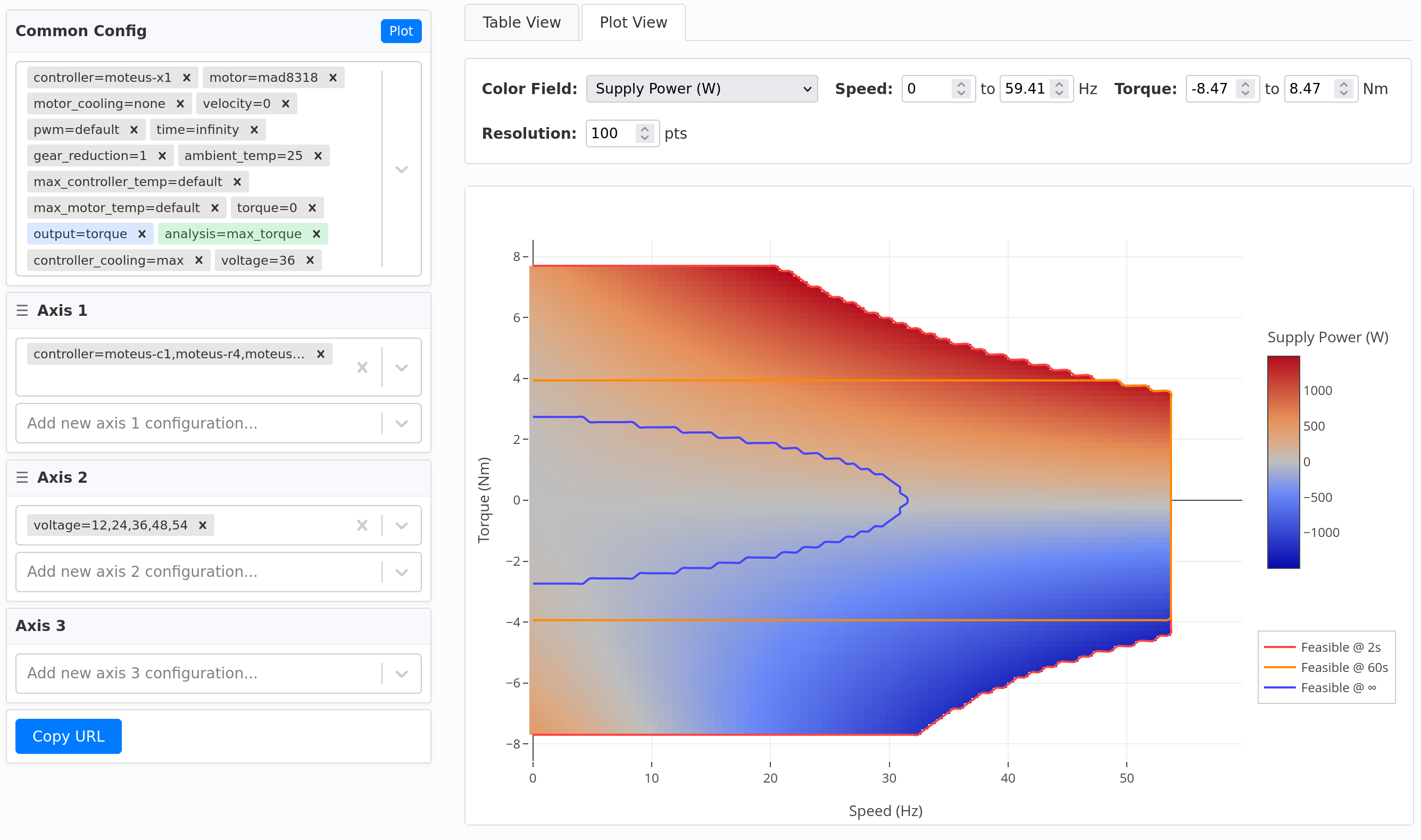
This is a 2d heatmap plot drawn between speed and torque, where the color plot can be one of supply power, efficiency, or motor or controller temperature at a number of fixed time periods. Additionally, the feasibility region for those fixed time periods (currently 2s, 60s, and infinity) are drawn as contour lines on top of the plot.
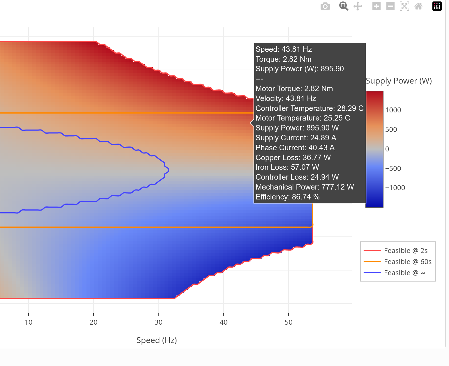
The mouse hover text shows the full operating point analysis for feasible regions:
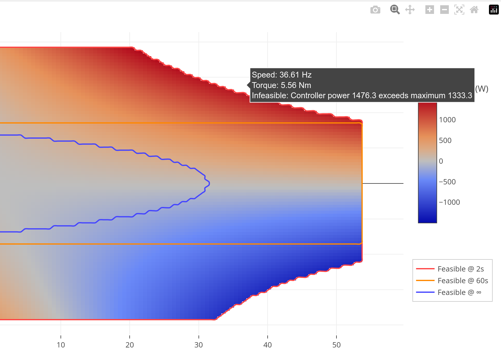
And for infeasible regions, the infeasibility reason is displayed in the hover text:
If the plot is active, then the “Copy URL” feature copies a link that renders that exact plot, which is a great way to share results and analyses with others.
Deployment
Given that this is strictly an improvement in capabilities, I’ve gone ahead and published it at the same URL as the original moteus Performance Analysis tool here.