Nonlinear encoder compensation with no reference
This post is part of series examining how low-cost off-axis encoders can be incorporated into a moteus controlled motor system. For the history, see the previous entries: part 1, part 2, part 3, and part 4. We left off after having tuned the bias current trimming of the MA600 in order provide output from the encoder itself. When compared against a reference AksIM-2, that left an error profile that looks like:
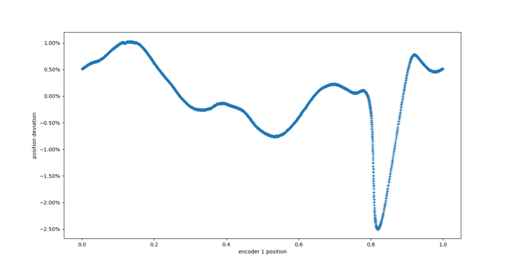
Position error with respect to AksIM-2 after BCT tuning
We can remove some of this remaining error using an table based approach on the moteus itself, and ideally can do so to a degree without requiring an external reference. The principle I’m going to use is similar to that used for the [measure_ma732_bct.py](https://github.com/mjbots/moteus/blob/main/utils/measure_ma732_bct.py) tool. In that tool, the motor is spun at a fixed open loop electrical velocity in order to see what tuning results in the lowest standard measured velocity ripple. What I would like to do in this case is spin the motor at a higher speed, sufficient that angular inertia dampens out as much of the non-linearity in torque production, and then use the velocity histogram again. But instead of just minimizing the overall standard deviation of the histogram, use it to generate the compensation table itself.
The first task here is to get the motor spinning at a moderately high speed with as little torque ripple as we can. The measure_ma732_bct.py step did not use FOC, and thus did not require that the motor be calibrated. However, spinning up a motor in locked in mode does generate a *lot* of torque ripple. We can do better, because just performing the BCT optimization gets the encoder “good enough” in all cases I’ve tested to successfully calibrate with moteus_tool -t 1 --calibrate. That means that we can use something like a fixed Q axis voltage in order to achieve a reasonably constant speed without having to worry about any PID tuning at all.
[Sidebar #1: To make –calibrate work with typical off-axis configurations, the moteus firmware as of 2024-10-29 now linearly interpolates compensation table mappings, whereas previously it did not].
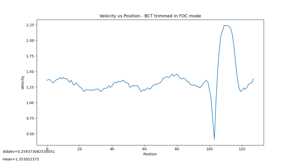
With the MA600 having been tuned per the above process and –calibrate run, and with the GL80 operating at a fixed Q axis voltage of 0.8V, the velocity histogram now looks like:
My idea is that the derivative of the position error in the encoder will roughly equal this measured histogram. Thus we can integrate it in order to derive the correct encoder compensation table. That result looks like the following:
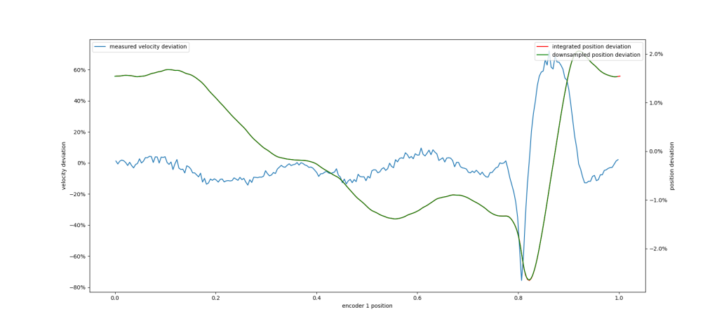
Note, the recovered integrated velocity error is not a superb fit for the initial error plot. However, we can apply it to the compensation table and see what we get. If only a single encoder is attached, and the compensation table is updated, it necessarily invalidates the commutation calibration, thus another pass at moteus_tool -t 1 --calibrate will be required.
[Sidebar #2: Prior to firmware 2024-10-29, moteus only supported 32 bin encoder compensation tables. In that revision, the table size was upgraded to 256 bins, which is necessary for the table size to not be the limiting performance factor in cases like this.]
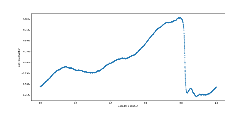
Position error compared to AksIM-2 after one round of inertial compensation
So yes, better, but not incredibly so. However, the remaining error is better behaved, which will result in less torque ripple. Thus if this compensated table is used to repeat the process, improved performance can result. In my approach, the integrated position error is used to adjust the current compensation with a less than unity heuristic, in order to approach, but not overshoot the final value so that it can be applied iteratively, i.e. over and over again. The maximum and standard deviation of the position error with respect to the reference AksIM-2 after different rounds of this compensation procedure are shown below, compared to a calibration calculated directly from the reference encoder:
| Round | Stddev position error | Max position error |
|---|---|---|
| 0 (just BCT tuning) | 0.704% | 2.496% |
| 1 | 0.523% | 1.034% |
| 2 | 0.354% | 0.688% |
| 3 | 0.287% | 0.551% |
| 4 | 0.194% | 0.423% |
| 5 | 0.139% | 0.348% |
| 6 | 0.124% | 0.292% |
| Reference Calibration | 0.013% | 0.073% |
The final position accuracy plot after all 6 tested rounds of “inertial” compensation looks like this:
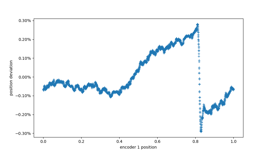
Position error compared to AksIM-2 after 6 rounds of inertial compensation
The standard deviation of the error is about 7x better than uncompensated, although still around 10x worse than directly calculating the compensation table from a reference encoder. Still, with this setup, that gives an absolute error of around 1.05 degrees, with a one sigma error of around 0.45 degrees. That is good enough for many applications.
In the next, and final, post in this series, I’ll give a run down of the process to provision a system using an off axis ring magnet encoder with the MA600.