Characterizing the MA600 off axis performance and tuning BCT
In previous iterations of this series (see part 1, part 2, and part 3), I built a breakout board for the MA600 TMR encoder and mounted it in an off axis configuration with a diametrically magnetized 32mm OD ring magnet along with a reference AksIM-2 encoder to compare against. Now we can finally get to the part where we can start looking at what the reported values look like.
For my first experiments, I set up a moteus-n1 with the AksIM-2 as the primary encoder, and the MA600 in motor_position.sources.1 in a slot that was not used for anything. Having done that, I plotted the difference in reported angle between the MA600 and the AksIM-2 through a full revolution below, using the compensate_encoder.py script that is now in the moteus repo in reference mode.
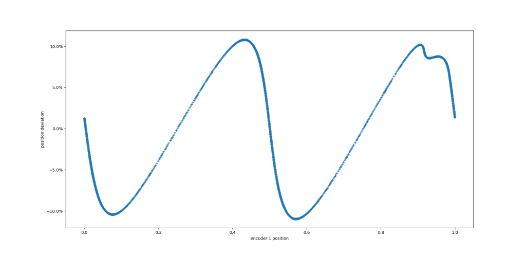
Off-axis MA600 position accuracy with no correction
So, yes, this is +- 10% error, which would be hard to use if uncorrected. To start with, lets work with the trimming capabilities built into the MA600 (and MA732/MA702). moteus has supported setting the “Bias Current Trimming” registers on the MA732 since firmware version 2024-06-17, and has supported it for the MA600 since MA600 support was first added in 2024-10-29. The MA600/MA732 datasheet have formulas to calculate an appropriate trimming value if the magnetic environment is known, or if the absolute error plot is known. However, I expect that many installations for moteus will use an off axis encoder as the sole encoder and will not necessarily have access to numerical values for the magnet properties. Thus, it would be nice to have a way to select the trimming values that relies on no a priori knowledge of the system.
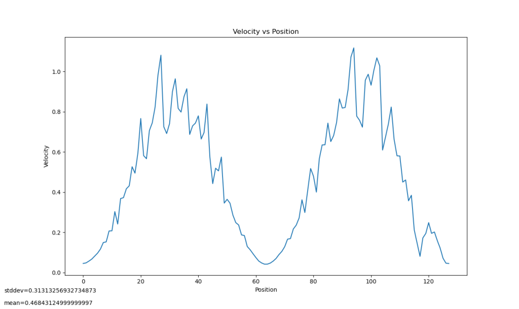
My concept, implemented now in [measure_ma732_bct.py](https://github.com/mjbots/moteus/blob/main/utils/measure_ma732_bct.py), is to attempt to spin the motor at a relatively constant velocity in an open loop “locked in” manner. While that is spinning, an on-device histogram of measured velocity vs position is recorded. The thought is that if the trimming is optimal, and the reported position is maximally linear, then the velocity profile will be as close to a straight line as possible. For example, the velocity histogram in this untrimmed state looks like this:
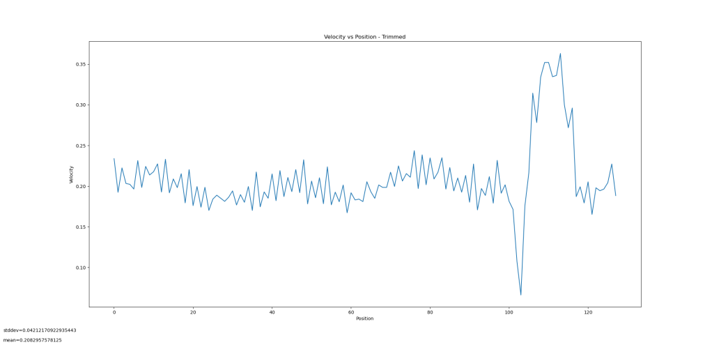
Where the histogram when the trimming has been optimally set looks like:
The principle of operation for measure_ma732_bct.py is to search over all possible trimming values, and find the one where the velocity profile has the minimum standard deviation, assuming that will be pretty close to optimal. Here is a plot of that standard deviation versus trim value for one run.
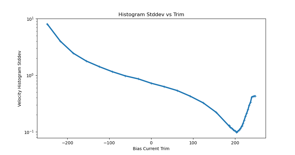
You can see that the optimal trim value of 204 is pretty near a global minimum, although the metric is relatively flat in that region (the plot above is on a logarithmic scale) so the exact value is probably not very critical within a few LSB.
To see where we’re at with just bias current trimming, here is a plot from compensate_encoder.py comparing against the reference AksIM-2 at this point.
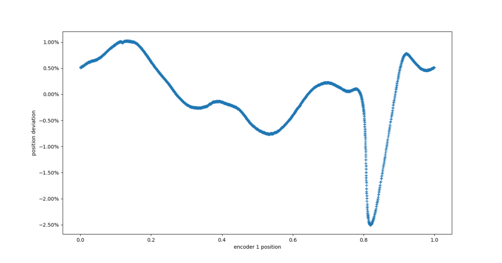
So yes, this is much improved over the baseline case with an average error more in the 0.5% instead of 5% in the untrimmed case. In the next post, I’ll look at approaches to remove more of this error while still not needing an actual reference.